PID control and PID algorithms are a complicated topic that are a bit difficult to understand. I’m going to try to explain it as it relates to the robot I just did and hopefully it will give you a general idea of what a PID algorithm is and why it is used.
To start off, some definitions. First, an algorithm for our purposes can be defined as a step-by-step procedure for solving a problem or accomplishing some end especially by a computer. The end we want to accomplish is making a robot balance on two wheels, and the PID part is a type of algorithm that follows certain steps in order to make that happen. Next, PID stands for Proportional-Integral-Derivative. The integral and derivative part are related to calculus, but if you haven’t taken calculus you can still understand and use PID controllers.
If you Google PID algorithms you usually turn up some funky looking diagrams like this:
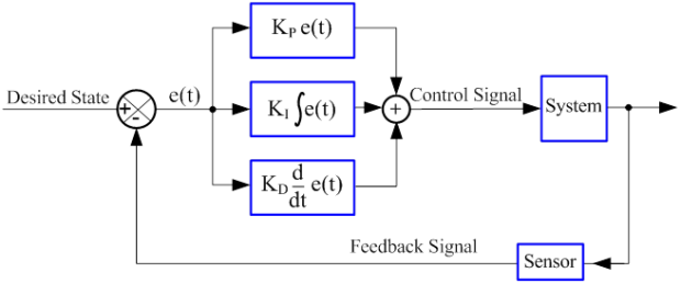
PID Control
From left to right:
- The desired state is the position you want your robot to be in. In the case of the balancing robot, that would be straight up and down.
- The e(t) part is the error experienced. So if you want your robot perpendicular to the surface it is on, i.e. 90 degrees, and it is actually 95 degrees, then e(t) is 5 degrees. The MPU-6050 tells you what orientation the robot is in, and you set the value for up and down in code. My robot worked on a value of 181 degrees. This is because I mounted the MPU-6050 parallel to the floor. That’s why I recommend setting up small programs to run each piece individually, because I was able to tell what value I was supposed to get without a lot of trial and error.
- The Kp * e(t) part is the Proportional part. explained later.
- The Ki * integral e(t) part is the Integral part. Later.
- The Kd * d/dt e(t) part is the Derivative part. You guessed it, later.
- The + means they are all added together into a control signal that is passed on to the system. In our case the system is a self balancing robot. The control signal tells the Arduino how fast to move the motors in order to balance the robot.
- Finally the sensor (the MPU-6050 in our case) sends the new current position of the robot back to the Arduino, which calculates the error and does the whole process again. This is called feedback, and makes this type of control loop a closed-loop system (as opposed to an open-loop system, which is easier but much less accurate).
The proportional term (gain) makes a change to the output that is proportional to the current error value. Larger values typically mean faster response since the larger the error, the larger the Proportional term correction signal. However, an excessively large proportional gain will lead to instability and oscillation. In layman’s terms, the further away from the desired state the robot is in, the larger the proportional term will need to be to correct it. So if your robot is wobbling a lot or is very off balance, you might need a larger Kp term to offset that because the robot is going to be further off balance. Here is a picture on what certain Kp values might look like:
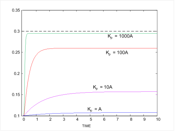
So A is e(t), and the value before A is the Kp value. You can see that larger values of Kp help the system achieve stability faster. However, you can overdo it. Too much Kp will give severe oscillations, as seen here:

Note that these Kp values are NOT recommended values for your robot, they are general values only to illustrate a point. My actual Kp value for the balancing robot was 40. Less than that gave a sluggish robot that oscillated wildly, while more than that was too aggressive an approach (like the 100000A example above). The original Franko robot had a value of 70. It all depends on the robot, even two robots that have the same purpose.
In engineering talk, the Integral term is proportional to the amount of time the error is present. The integral term accelerates the movement of the process towards the set value and eliminates any residual steady-state error that occurs with a proportional only controller. The contribution from the integral term is dependent both on the magnitude of the error and on the duration of the error.
What that means is that robots are only as accurate as you program them to be, and as accurate as their motors are. Without going into detail, just because you program the robot to turn a wheel a certain amount doesn’t mean it will turn that exact amount. Usually it will be a little off (due to friction, motor deadzones, power losses, etc.). The integral term (Ki) takes this error and adds it up until it is large enough to make a difference.
For example, if the MPU should read 181 degrees to be balanced, but reads 181.1, that might not be enough to move the motors enough to correct for that .1 difference. But if the MPU reads that value 100 times in a second, the extra .1 degree becomes 10 degrees of cumulative error, and that IS enough to move the motors.
This can have negative consequences if the Ki error is too large though, as shown here:
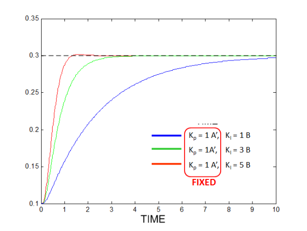
Ki Values
In this graph, B is e(t) and the number before B is Ki. For the balancing robot, a large Ki will enable it to steady itself very quickly, and will help eliminate drift. If you look up videos of balancing robots on YouTube you will see that a lot of them will roll around. That is because of their steady state error, and a larger Ki will stop that (as long as it’s not too large). Mine was set at 500, which is over 7 times greater than the Kp value.
Finally is the Kd term. With the derivative term, the controller output is proportional to the rate of change of the measurement or error. The derivative term slows the rate of change of the controller output, most notably near the controller set value. It therefore reduces the magnitude of the overshoot produced by the integral component and improves stability. Larger Kd values decrease overshoot, but slows down transient response and may lead to instability from signal noise amplification from differentiation of the error.
To translate, the Kd term helps the Kp term not overshoot the mark and reduces oscillations. Too large of a Kd term will slow down the response of the robot and make it slower to balance, while too small of a Kd term will make it shake a lot. Mine was set at 1.9, so much smaller than either the Kp or Ki terms.
Also I was using the auto tune function of the PID library, and so I do not know the actual final values of the 3 constants. The way I set them got me good enough results so that the auto tune could “fix” them and get the robot to balance well. Some more trial and error without the auto tune will be necessary to get good performance without the warm-up jitters that are shown in the video posted previously.
Note that all of the “engineer” talk and the graphs came from a presentation from my college instrumentation course that I am unable to link to because it is behind a username/password sign in.
Obviously PID algorithms are complex and are different for each robot you will build. Hopefully this brief overview gives some insight into how one goes about constructing a PID algorithm.
 I Just don’t get the post office sometimes. Usually I have no problems with them. Packages arrive on time and are sent in a timely manner with no issues. Unfortunately that was not the case for the last package I ordered.

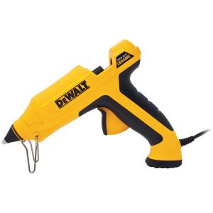 Enter hot glue. This substance is really just a sticky thermoplastic with a very low melting point. It’s fed into a “gun” that lets you squirt it wherever you want. It has some fabulous properties for robot prototyping. For starters, the glue dries quickly so you can fix a couple of wires in place with minimal time and fuss. The glue also has good holding power, so things that you glue will stay in place. I even glued the IMU onto the robot for the self balancing robot I made, and it never fell off even with all the gyrating that robot did. However, the glue is paradoxically rather easy to remove. Just grab a blob with your fingers and pull and it comes right off usually. And if it doesn’t, a little work with the back of a razor blade or xacto knife will scrape it right off.


